July 2026: High Dimensions and Tidymodels

This post covers the second month of development for the classbound package. July focused on three main goals. I solved the memory problems for high-dimensional data. I integrated the package with the tidymodels ecosystem. I improved the interactive Shiny application for model comparison.

Idiomatic Architecture

I began the month by refactoring the package architecture. The package uses native R S3 dispatch instead of string-based method routing.

Users no longer pass a string to the fit function. They pass the classifier function. The package handles the rest. This design pattern aligns with standard R conventions.

I built a default prediction adapter. This adapter handles standard R models that return vectors or factors. This change removes the need for custom adapters for most classifiers.

For classifiers that return complex list objects, I introduced the predfun fallback. This mechanism allows the core pipeline to extract predictions without failing. The package is easier to extend and maintain. I also refactored the model object to nest the features and class levels inside a specific metadata list. This prevents namespace collisions with third-party model wrappers.

I also hardened the package’s object-oriented design by introducing the classbound_multi S3 subclass. Previously, single and multi-model objects shared the exact same class, which forced downstream functions into defensive branching. By delegating this logic to R’s native C-level S3 dispatcher, the internal pipeline remains strictly polymorphic and extensible.

Solving High-Dimensional Memory Limits

In June, grid generation caused memory crashes for data with many features. A dense grid for high-dimensional data requires too much memory. The system attempts to calculate predictions for every possible combination of values. This causes a combinatorial explosion.

I solved this problem. I implemented an inverse projection strategy. The boundary_compute() function accepts a projection object. The function generates a sparse two-dimensional grid. It maps this grid back into the high-dimensional space.

graph TD
    A[High-Dimensional Data] --> B[Generate Projection Object]
    B --> C[Create 2D Grid]
    C --> D[Map Grid to High Dimensions]
    D --> E[Compute Predictions]
    E --> F[Plot Boundary]

This approach computes boundaries without creating large grids. It solves the memory explosion problem. I also added fixed-value slicing. Users can generate a two-dimensional slice of a multi-dimensional space. The function imputes missing numeric features with the median value. It imputes missing categorical features with the mode. Users can override these defaults with custom reference values.

# Compute a 2D slice of a 4D random forest model
model_slice <- boundary_compute(
  model_rf_4d, 
  range = list(bill_length_mm = c(30, 60), bill_depth_mm = c(12, 22)),
  reference = list(flipper_length_mm = 200, body_mass_g = 4000),
  resolution = 300
)

plot(model_slice)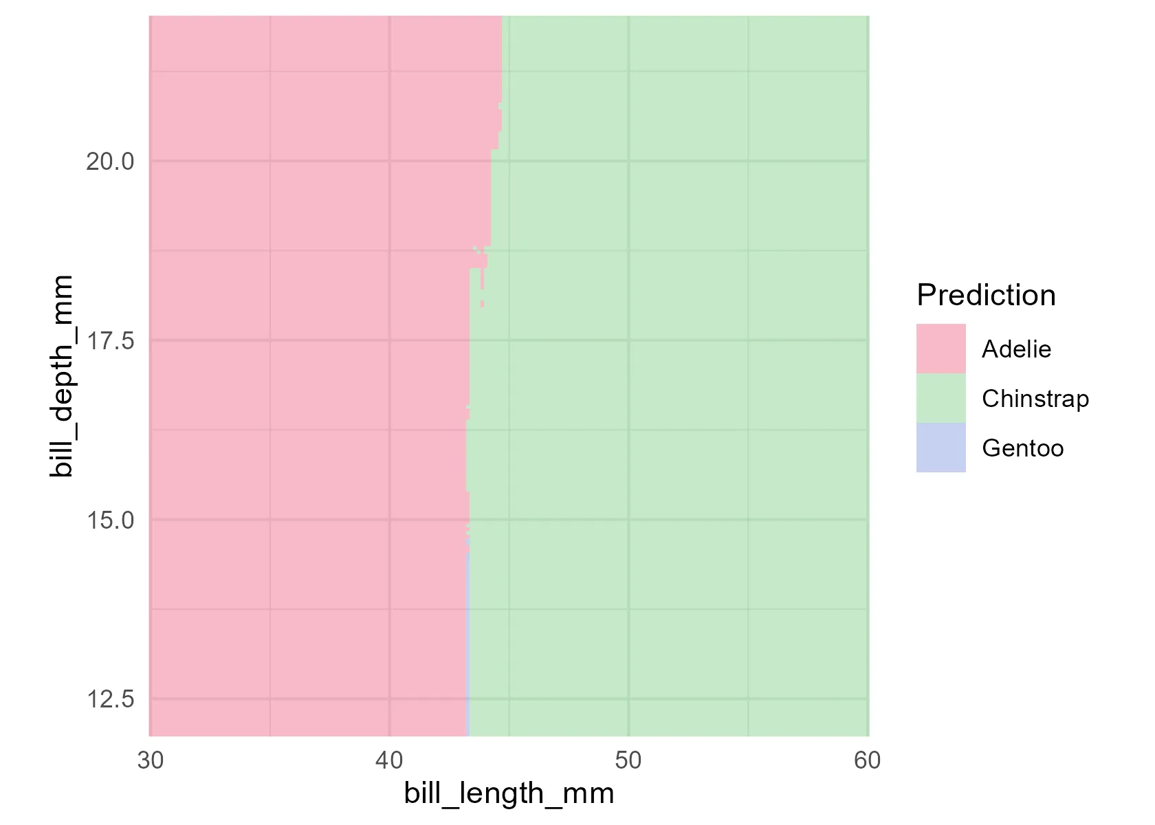

Integrating Tidymodels

I integrated classbound with the tidymodels ecosystem. I maintained strict backend independence. The core pipeline remains agnostic to the modeling framework.

I created the as_classbound() generic function. This allows users to bring their pre-fitted models into the pipeline. They do not need to refit their models.

I built adapters for workflow and model_fit objects. I built a wrapper for workflow_set objects. This allows users to orchestrate boundary extraction for entire sets of models at once.

graph LR
    A[tidymodels workflow] --> B(as_classbound)
    C[parsnip model_fit] --> B
    D[workflow_set] --> E(boundary_workflow_set)
    B --> F[classbound object]
    E --> G[classbound_multi object]

# Compute boundaries directly on an unfitted workflow set
multi_model <- boundary_workflow_set(
  wf_set, 
  data = data, 
  range = list(bill_length_mm = c(30, 60), bill_depth_mm = c(12, 22)),
  response = "species",
  resolution = 300
)

plot(multi_model)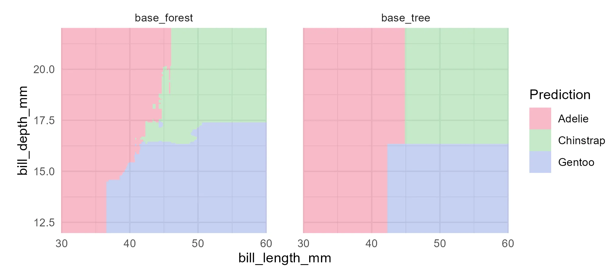

Multi-Model Comparisons

Comparing decision boundaries of different classifiers was a priority. I extended the package to handle multiple models in a single object.

The boundary_compute() function accepts a list of classbound objects. It computes the grid once. It validates the feature sets. It returns a unified classbound_multi object.

library(rpart)
library(randomForest)

# Fit competing models on the Palmer Penguins dataset
model_tree <- fit_model(penguins_data, species ~ ., rpart)
model_rf <- fit_model(penguins_data, species ~ ., randomForest)

# Compute unified multi-model boundaries
multi_bound <- boundary_compute(list(model_tree, model_rf), resolution = 300)
plot(multi_bound)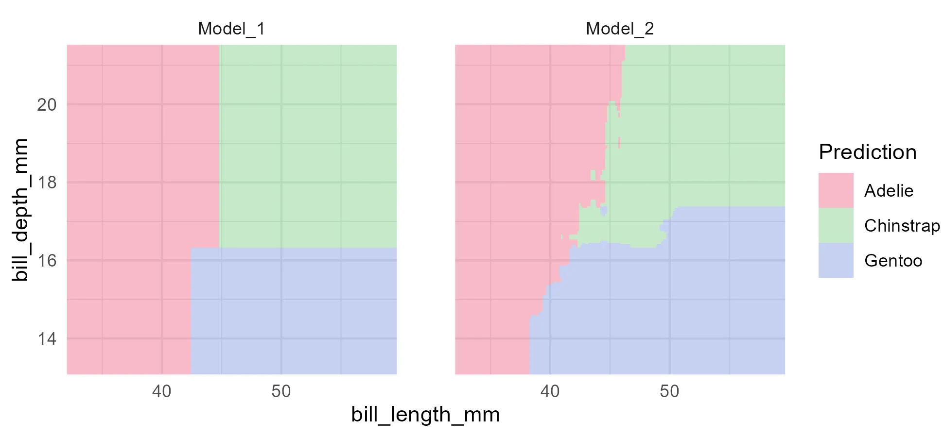

This visual output demonstrates the utility of the package. It compares the rigid, orthogonal splits of a decision tree against the flexible margins of a random forest on non-linear data.

I also added a disagreement map. This feature reveals where algorithms produce conflicting predictions.

# Plot the disagreement map
plot(multi_bound, type = "disagreement")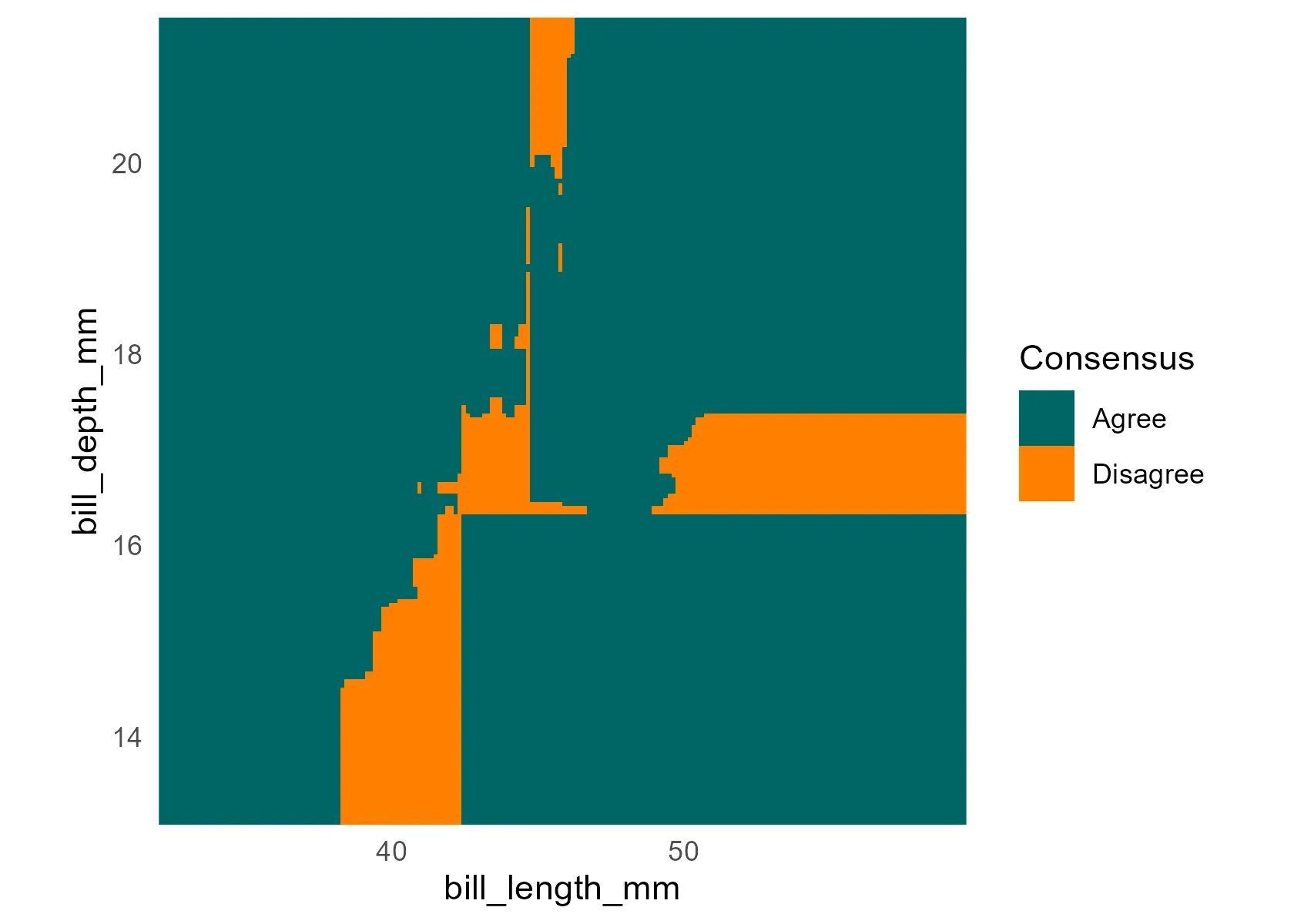

The disagreement map overlays points to show consensus and conflict. It provides a visual comparison of model logic. The green points highlight the exact spatial regions where the two algorithms disagree on the class assignment.

I also introduced a show_gradient toggle. Users can disable the probability surfaces. This renders flat, solid boundaries. Previously, the package auto-detected probability support and forced gradient rendering. This new toggle provides explicit user control.

model_rf_single <- boundary_compute(model_rf, resolution = 300)

# Render hard boundaries without probability gradients
plot(model_rf_single, show_gradient = FALSE)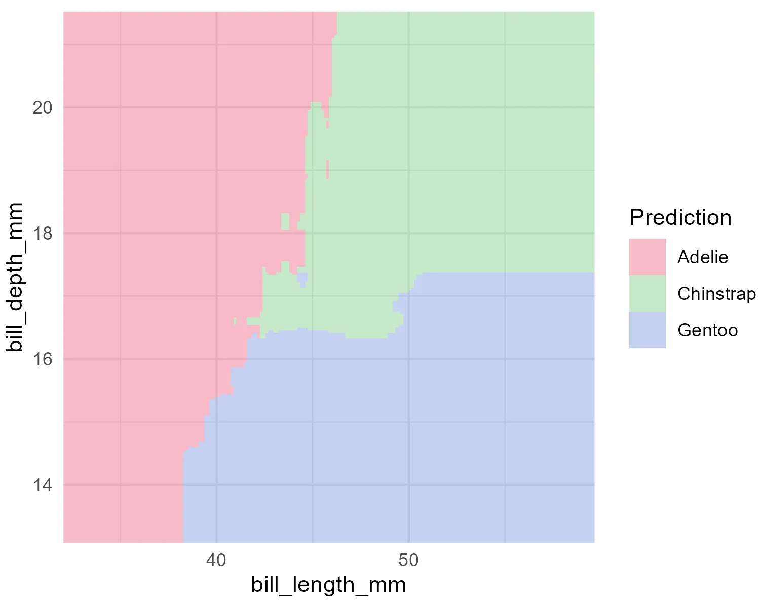

High-Dimensional Projection

When modeling data with more than two features, generating a meaningful 2D visualization requires mathematical projection. The package now fully supports mapping complex boundaries onto any custom 2D plane using a projection matrix, such as the output of Principal Component Analysis (PCA).

# Extract the 4 numeric features from Palmer Penguins
penguins_data <- na.omit(penguins[, c("species", "bill_length_mm", "bill_depth_mm", "flipper_length_mm", "body_mass_g")])

# Fit a Random Forest on all 4 dimensions
mm <- fit_model(penguins_data, species ~ ., randomForest, interface = "formula")

# Compute the PCA projection basis
pc <- prcomp(penguins_data[, -1], center = TRUE, scale = TRUE)

# Compute the boundary on the PC1 x PC2 plane
grid_data <- boundary_compute(
  model = mm, 
  range = list(PC1 = c(-4, 4), PC2 = c(-4, 4)), 
  resolution = 200, 
  projection = list(basis = pc$rotation[, 1:2], center = pc$center, scale = pc$scale)
)

# Render the projected boundary and data points
plot_boundary(grid_data, obs_data = penguins_data, true_label = "species")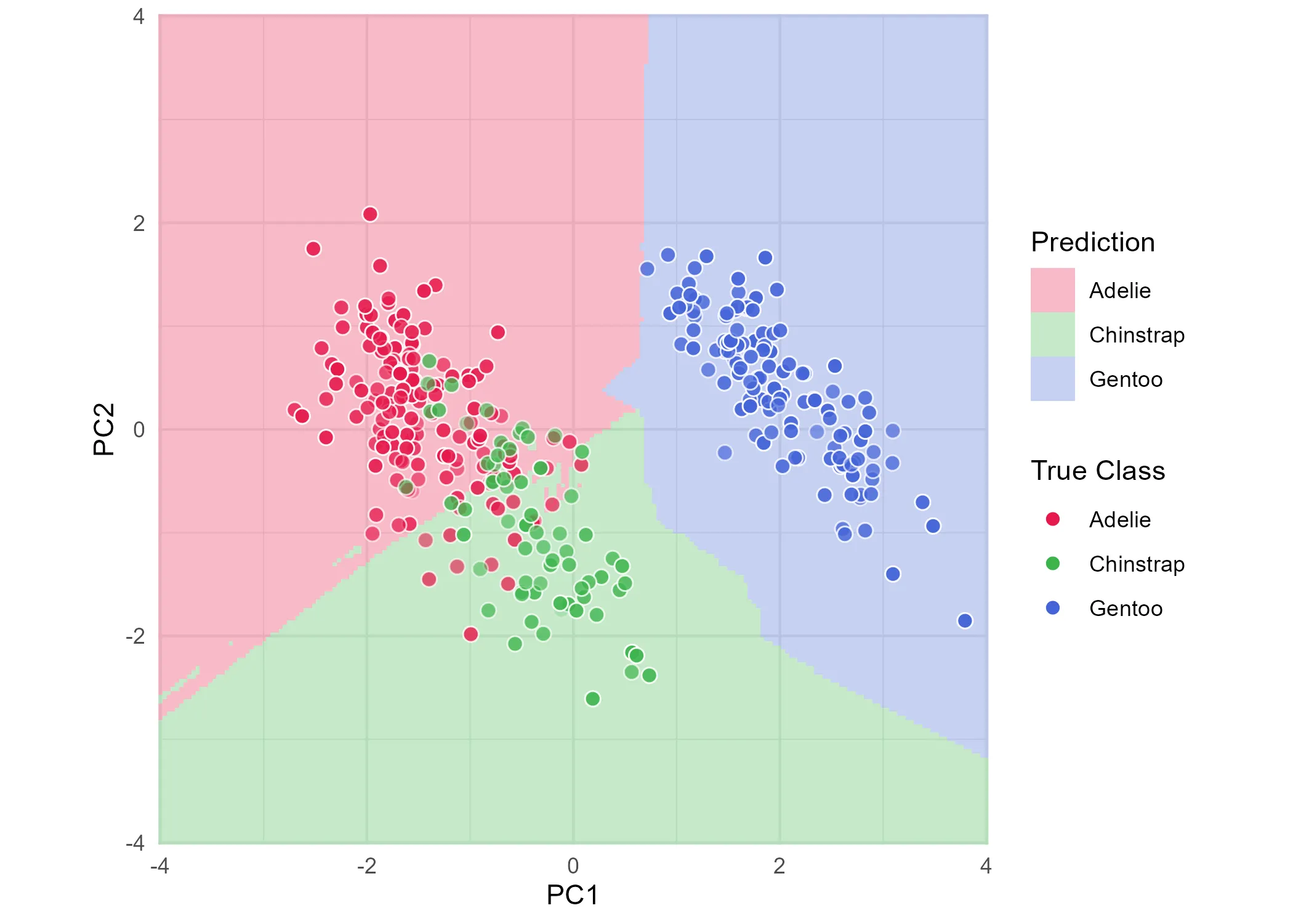

Interactive Shiny Application

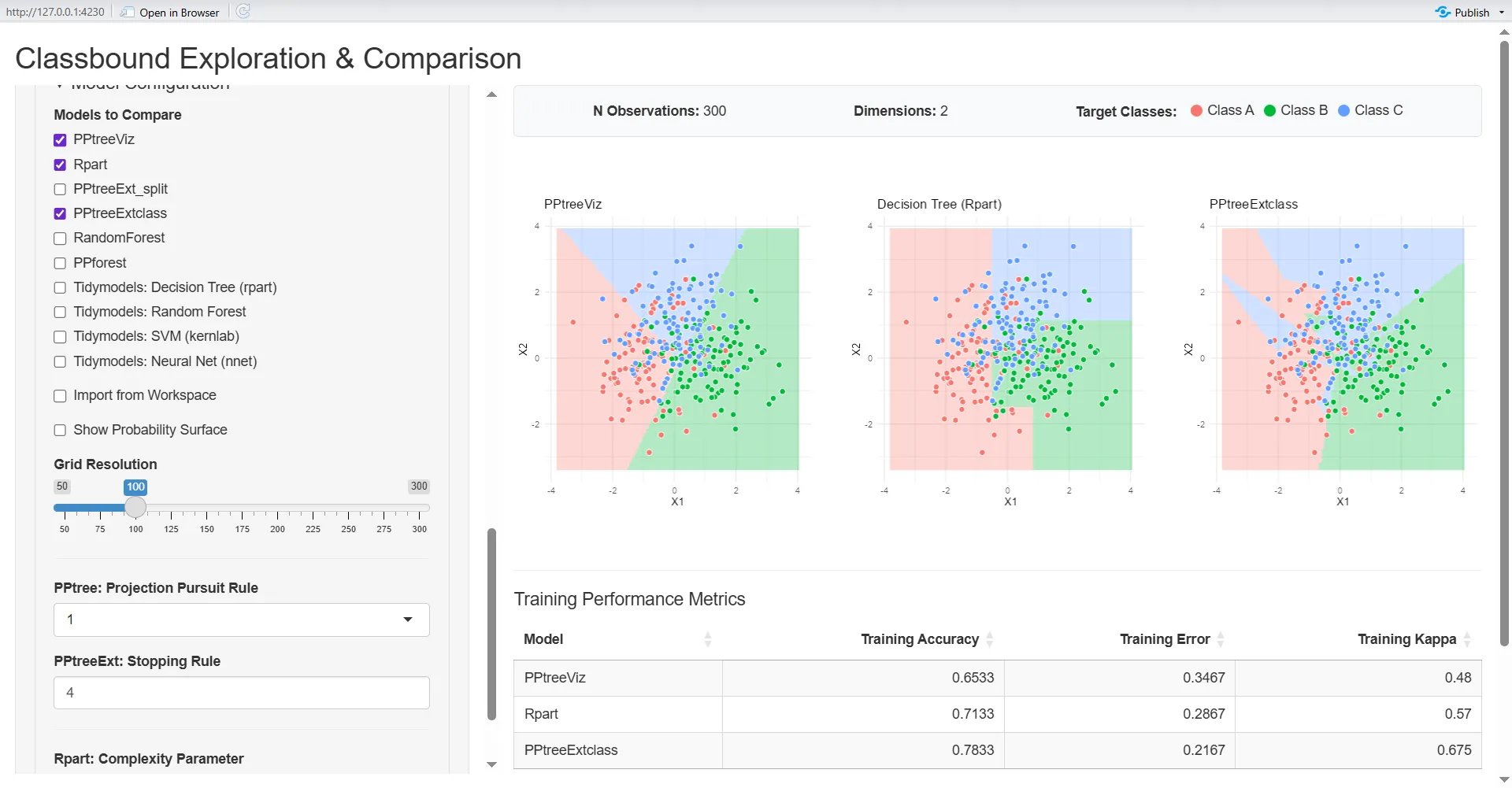
I built a complete interactive Shiny application. This interface consumes the core package functions without duplicating logic. It provides a standalone environment for visual analysis.

I added specific capabilities to improve the tool:

• Performance Metrics: A data table displays training accuracy, error rates, and Kappa statistics.
• Grid Resolution: A slider sets the boundary evaluation density. Users control the computational load.
• Workspace Import: The tool captures workflow, model_fit, and model_spec objects from the active R session. Users compare models without writing code.
• Tour Steering: An interpolation slider moves the projection between orthogonal bases. Users traverse high-dimensional spaces.
• Extended Support: The application supports PPforest models.
• Error Handling: The interface shows model failures as popup notifications. I corrected the PCA math to handle zero-variance features during simulation.

I also enforced mathematical rules during preprocessing. The pipeline rejects datasets with fewer than two rows. It blocks infinite values. These rules prevent C++ errors in the underlying classifier packages.

Next Steps

August covers the final touches to the package. The primary objectives are comprehensive testing and finalizing the documentation. I will build test suites to cover all integration points.